Generating waveforms

Training data for Dingo consist of pairs of parameters \(\theta\) and corresponding simulated strain data sets \(d_I\), where \(I\) runs over the GW interferometers (L1, H1, V1, etc.). Additionally, when conditioning on detector noise properties, data also include noise context (the PSD \(S_{\text{n},I}\)). Strain data sets are of the form

\[ d_I = h_I(\theta) + n_I, \]

where \(h_I(\theta)\) is a signal waveform (provided by a waveform model) and \(n_I\) is a noise realization (stationary and Gaussian, consistent with \(S_{\text{n}, I}\)).

Data domain

At present, Dingo works entirely with frequency domain data. Although NPE is very flexible and could in principle learn to interpret data in any representation, FD data are especially convenient because (1) stationary Gaussian noise is independent in each frequency bin, so noise generation is straightforward, (2) time shifts take a simple form, enabling improved data augmentation, and (3) the noise context is already in FD. Other domains could be useful in the future, however, so the code is written in a way that the domain could be adapted.

The domain is specified by instantiating a UniformFrequencyDomain,

import warnings
warnings.filterwarnings("ignore", "Wswiglal-redir-stdio")
import lal

from dingo.gw.domains import UniformFrequencyDomain
domain = UniformFrequencyDomain(f_min=20.0, f_max=1024.0, delta_f=0.125)

Derived class properties include, e.g., the frequency grid. Frequency arrays run from 0 to f_max, as is standard for GW data analysis software.

domain.sample_frequencies

array([0.000000e+00, 1.250000e-01, 2.500000e-01, ..., 1.023750e+03,
       1.023875e+03, 1.024000e+03], dtype=float32)

Note

The standard deviation of white noise in each frequency bin is stored in domain.noise_std. In frequency domain, this is given by \(\sqrt{1/4\delta f}\). See data conditioning for details.

Various class methods also act on data, to perform operations such as zeroing below f_min, truncating above f_max, or applying a time shift:

Waveform generator

Waveforms are generated using the WaveformGenerator class (or its subclass NewInterfaceWaveformGenerator, for employing the new LIGO waveform interface, needed for some approximants). This depends on a Domain as well as a waveform approximant and a reference frequency f_ref. In the backend, the WaveformGenerator class calls LALSimulation functions (typically SimInspiralFD) via the SWIG-Python interface. For time domain waveforms, SimInspiralFD takes care of FFTing to frequency domain. The NewInterfaceWaveformGenerator class calls the gwsignal module, a Python interface recently implemented in LALSimulation, which is needed for employing some of the latest waveform approximants, as the SEOBNRv5HM and SEOBNRv5PHM.

from dingo.gw.waveform_generator import WaveformGenerator #, NewInterfaceWaveformGenerator

wfg = WaveformGenerator(approximant='IMRPhenomXPHM', domain=domain, f_ref=20.0)
# wfg = NewInterfaceWaveformGenerator(approximant='SEOBNRv5PHM', domain=domain, f_ref=20.0)

Setting spin_conversion_phase = None. Using phase parameter for conversion to cartesian spins.

To generate a waveform we first need to choose parameters. Here we sample parameters from a bilby.core.prior.PriorDict. We use the default Dingo intrinsic prior.

from bilby.core.prior import PriorDict
from dingo.gw.prior import default_intrinsic_dict

prior = PriorDict(default_intrinsic_dict)
prior

{'mass_1': Constraint(minimum=10.0, maximum=80.0, name=None, latex_label=None, unit=None),
 'mass_2': Constraint(minimum=10.0, maximum=80.0, name=None, latex_label=None, unit=None),
 'mass_ratio': bilby.gw.prior.UniformInComponentsMassRatio(minimum=0.125, maximum=1.0, name='mass_ratio', latex_label='$q$', unit=None, boundary=None, equal_mass=False),
 'chirp_mass': bilby.gw.prior.UniformInComponentsChirpMass(minimum=25.0, maximum=100.0, name='chirp_mass', latex_label='$\\mathcal{M}$', unit=None, boundary=None),
 'luminosity_distance': DeltaFunction(peak=1000.0, name=None, latex_label=None, unit=None),
 'theta_jn': Sine(minimum=0.0, maximum=3.141592653589793, name=None, latex_label=None, unit=None, boundary=None),
 'phase': Uniform(minimum=0.0, maximum=6.283185307179586, name=None, latex_label=None, unit=None, boundary='periodic'),
 'a_1': Uniform(minimum=0.0, maximum=0.99, name=None, latex_label=None, unit=None, boundary=None),
 'a_2': Uniform(minimum=0.0, maximum=0.99, name=None, latex_label=None, unit=None, boundary=None),
 'tilt_1': Sine(minimum=0.0, maximum=3.141592653589793, name=None, latex_label=None, unit=None, boundary=None),
 'tilt_2': Sine(minimum=0.0, maximum=3.141592653589793, name=None, latex_label=None, unit=None, boundary=None),
 'phi_12': Uniform(minimum=0.0, maximum=6.283185307179586, name=None, latex_label=None, unit=None, boundary='periodic'),
 'phi_jl': Uniform(minimum=0.0, maximum=6.283185307179586, name=None, latex_label=None, unit=None, boundary='periodic'),
 'geocent_time': DeltaFunction(peak=0.0, name=None, latex_label=None, unit=None)}

p = prior.sample()
p

{'mass_ratio': 0.134488607823063,
 'chirp_mass': 72.68826723349574,
 'luminosity_distance': 1000.0,
 'theta_jn': 2.115774264754338,
 'phase': 6.277423673741555,
 'a_1': 0.05488692077019725,
 'a_2': 0.17569595065281166,
 'tilt_1': 1.2836247952488415,
 'tilt_2': 2.8253930297013174,
 'phi_12': 5.380242374015733,
 'phi_jl': 6.228059574343675,
 'geocent_time': 0.0}

Finally, we generate the waveform. This is returned as a dictionary, with entries for each polarization. This way of representing a sample is used throughout Dingo, and will be very convenient when applying transforms (to apply extrinsic parameters, add noise, etc.).

h = wfg.generate_hplus_hcross(p)
h

{'h_plus': array([0.+0.j, 0.+0.j, 0.+0.j, ..., 0.+0.j, 0.+0.j, 0.+0.j]),
 'h_cross': array([0.+0.j, 0.+0.j, 0.+0.j, ..., 0.+0.j, 0.+0.j, 0.+0.j])}

import matplotlib.pyplot as plt
plt.plot(domain.sample_frequencies, h['h_plus'].real, label='real')
plt.plot(domain.sample_frequencies, h['h_plus'].imag, label='imag')
plt.xlim((10,1024))
plt.xscale('log')
plt.legend()
plt.xlabel('f')
plt.ylabel(r'$h_+$')
plt.show()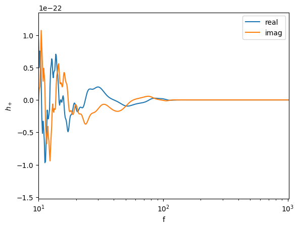

Note that the waveform is nonzero slightly below f_min. This simply arises from the model implementation in LALSimulation. When training networks, input data will be truncated below f_min.

The complete specification of the WaveformGenerator class is given as

Waveform modes

Add later.